At the beginning of this summer, I embarked on the journey of learning about the ephemeral nature of life (or, quantum field theory), as a mean of exercising the mind if you will, so that I won’t start off the new semester having to resort to google to remind myself what Newton’s second was. Much of what I already knew doesn’t go much further than a qualitative understanding that is enough to ‘wow’ some laymen at a party. Having read Susskind’s book on Special Relativity and Classical Field Theory, I started reading A. Zee’s Quantum Theory in a Nutshell in order to have a firmer grasp of the mathematical nitty-gritty of QFT.
Zee’s approach to establishing a quantum theory of fields is quite modern. The ‘classical’ texts on QFT usually take a route to canonically quantise what we know about field, where Zee gives it the path integral treatment. Say we want to travel from point A to B. We are free to choose whatever path we want, but we’d prefer an easier path should there be one. The path integral formalism is akin to integrating over all possible paths, but by the principle of least action, certain paths that minimise the action $S$, has a higher amplitude and are therefore weighted more. A very nice feature of this formalism is that through the use of Wick’s theorem in the computation of the integrals, Feynman diagrams just seem to fall in place, as a mean to keep track of the cross terms of the functional derivatives.
Another route, which I prefer, is canonical quantisation. It is demonstrably clearer than some aspects of the path integral treatment in a way that when you derive the quantisation canonically, you know that you are in a quantum regime, whereas the feeling is somewhat absent in the case of the path integral derivations. One begins with the Canonical Commutation Relation i.e.: \[[\hat p, \hat q] = -i\].
Quantum harmonic oscillator
Quantum harmonic oscillators underpin QFT, and unsurprisingly, much of quantum theory. Here I give a review of the derivation of QHO from classical Hamiltonian dynamics, and aim to show how doing this will help us to establish QFT. One may rightfully ask: well, if we put all our eggs in one basket, namely that of the ‘harmonic potential’ basket, what if we have an anharmonic potential? Indeed, as soon as we deviate from the harmonic potential, this ‘toy model’ of ours will no longer produce results that agree with reality, i.e. within the proton when there’s a positively non-zero quartic interaction potential term. The solution that physicists came up with is, of course, perturbation theory. Such imperfection manifests itself differently when we take the two routes of quantisation. For the path integral formalism, this presents an unsolvable integral with a quartic term in the Lagrangian in the exponential.
We know from classical mechanics, that the Hamiltonian of a system is:
\[\mathcal{H}= \frac{p^2}{2}+V(q)\]
where we have set $m = 1$ and use $q$ in lieu of $x$ as the variable for position, a convention in field theories.
For a harmonic potential $V$, we can express $\mathcal{H}$ as:
\[\mathcal{H} = \frac{p^2}{2}+\frac{\omega^2}{2}q^2\]
and because we have set mass to be unitary, the time derivative of position is just momentum.
\[\dot q = p\]
We can find the force on the system, which follows the relation:
\[\dot p = – \pdv{V}{q} = – \omega q\]
\[\ddot{q} = – \omega q\]
We can remind ourselves of the 1D TDSE:
\[i \hbar \pdv{\psi}{t} = – \frac{\hbar^2}{2}\pdv[2]{\psi}{x}+\frac{\omega^2}{2}x^2\]
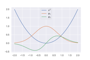
From just looking at the partial differential equation, we can choose an appropriate ansatz, namely the quadratic exponential function that oscillates within the constraint of the harmonic potential well.
To get around solving nasty differential equations, we can reformulate our Hamiltonian operator in the form of ladder operators. Sparing the algebraic proof, we can introduce a new operator and its hermitian conjugate for this purpose:
\[\hat a = \frac{1}{\sqrt{2\omega}} (\omega \hat q + i \hat p)\]
\[\hat{a}^\dagger = \frac{1}{\sqrt{2\omega}}(\omega\hat{q} – i \hat{p})\]
Note that $\hat a$ is positively not hermitian due to the presence of $i$. By rearranging to solve for $\hat p$ and $\hat q$, we can re-express our Hamiltonian operator:
\[\hat H = \omega (\hat a ^\dagger \hat a + \frac{1}{2})\]
With a little more algebra, we can show that the commutator for $\hat a$ and $\hat a^\dagger$ is 1.
For reasons that will soon be obvious, $\hat a^\dagger$ is called the raising or creation operator, and $\hat a$ is called the lowering or annihilation operator. Let us propose that the following is true:
\[\hat a^\dagger \ket{0} = \ket{1}\]
where $\ket{0}$ is the ground eigenstate (which is non-zero), and $\ket{1}$ is the eigenstate of the first energy level. For $\ket{1}$ to be an eigenstate of the Hamiltonian operator, $\ket{1}$ must satisfy the TISE:
\[\hat H \ket{1} = E_1 \ket{1}\]
substituting in what we proposed, we have:
\begin{align*}\hat H \ket{1} &=\omega (\hat a ^\dagger \hat a + \frac{1}{2})\hat a^\dagger \ket{0}\\ &=\omega \hat a^\dagger \hat a \hat a^\dagger \ket{0} + \frac{\omega}{2}\hat a^\dagger \ket{0}\end{align*}
Using what we know for the commutator of the operators, we show:
\[\hat H \ket{1} = \frac{3\omega}{2}\ket{1}\]
From here, it is a relatively treacherous path to show that the following vector will form the complete eigenbasis for the Hamiltonian operator:
\[\ket{n} = \frac{1}{\sqrt{n!}}(\hat{a}^{\dagger})^n \ket{0}\]
which means we can ‘create’ state we need from the ground state!
From particles to fields
We now have everything we need to quantise a Klein-Gordon field.
We can remind ourselves the Lagrangian for such a field:
\[\mathcal{L} = \frac{1}{2}\partial^\mu\varphi\partial_\mu\varphi-\frac{m^2}{2}\varphi^2\]
We can define some analogues for fields:
\[\pi = \pdv{\mathcal{L}}{\dot\varphi} = \dot\varphi\]
We can find the field operator $\hat \varphi$ in momentum space:
\[\hat \varphi(\vec x, t) – \int \frac{\dd[3]{k}}{(2\pi)^{3/2}\sqrt{2\omega_k}} \left [ \hat a(\vec k) e^{-i(\omega_k t – k^\mu x_\mu)} + \hat a^\dagger (\vec k) e^{i (\omega_k t – k^\mu x_\mu)}\right ]\]
as well as $\hat \pi$ in momentum space:
\[\hat \pi(\vec x, t ) = \partial_0 \hat \phi = \int \frac{\dd[3]{k}}{(2\pi)^{3/2}\sqrt{2\omega_k}}\left [ \hat a(\vec k) (-i\omega_k)e^{-i(\omega_k t – k^\mu x_\mu)} + \hat a^\dagger (\vec k)(i\omega_k) e^{i (\omega_k t – k^\mu x_\mu)}\right ]\]
Using $\hat \varphi$ and $\hat \pi$, we can find the Hamiltonian density:
\[\mathcal{H} = \frac{1}{2}\int \dd[3]{x} (\hat \pi^2 + (\nabla \hat \varphi)^2 + m^2 \hat\varphi^2)\]
We now have a jumbled mess of multiple integrals over multiple variables, but luckily, there’s only one term that is dependent on $x$. Namely:
\[\int \dd[3]x e^{i(\vec k + \vec l)\cdot\vec x} = (2\pi)^3 \delta^3(\vec k + \vec l)\]
where we have introduced a new vector $\vec l$ for the $\hat \pi$ integral.
All there is left to do now, is to take a deep breath, collect our terms, and put a hat on $H$!
\[ \hat H = \int \frac{\dd[3]{k}}{(2\pi)^{3/2}\sqrt{2\omega_k}} \left [ \frac{1}{2} + \hat{a}^\dagger (\vec k) \hat a (\vec k) \right ] \omega_k\]
et voilà, we have established a quantum theory for a Klein-Gordon free field with a harmonic potential! It is to be expected that our Hamiltonian would contain an integral over momentum space, such that we would have a separate Hamiltonian operator for every point in the field! And perhaps the most interesting thing to take away is the statement, what is a quantum field if not an infinite collection of quantum harmonic oscillators?
Damn all this stuff look real complicated and all. Many math-looking symbols and all, very nice.
Thank you very much for your kind comment.
Damn all this stuff look real complicated and all. Is this like quantum like really smart science and teleportation and stuff? cuz that’ll be real dope. btw you owe me 280 pounds.
Them stuff in there look complicated and all. Is this like quantum like really smart science and teleportation and stuff? cuz that’ll be real dope. btw you owe me 280 pounds.