This is the second instalment of my journey to learn Quantum Field Theory. This week, I got a preview at Renormalisation Theory and how we can use this to solve seemingly impossible physical problems, and during the process, I encountered a particularly peculiar sum…
Questionable Pedagogy…
I remember that in grade 10, my then maths teacher, Mr Prior, showed the class a ‘proof’ that the sum of all natural numbers is equal to negative one twelfth, i.e.:
\[\sum_{n=1}^\infty n = -\frac{1}{12}\]
Despite the fact that proof is in quotes, I am using the term very liberally. What seemed to be an impressive mathematical feat at the time, now seems like a dubious attempt to trick young minds (ok maybe that’s a bit much).
The proof starts by proposing the following sequence:
\[S_1 =((-1)^{n})_{n=0}^{\infty}= 1, -1, 1, -1,…\]
This sequence simply alternates between 1 and 0. Suppose we take an infinite sum of the sequence, what would be the final result? The video says, since the terms oscillate between 1 and 0, so depending on whether we stop at an even or odd indexed term, we would end up with either 0 or 1, respectively, so let’s take the average of those, and assign the value one half to the series:
\[\sum_{n=0}^\infty(-1)^n = \frac{1}{2}\]
Now this may seem reasonable, the 15-year-old me certainly thought so. But upon closer inspection, you would notice that this is indeed extremely cavalier and will open the Pandora’s box as a result. We can’t just assign a value to a positively non-converging series! But alas, we shall address these mathematical floppiness later on. The second series that we will need is:
\[S_2 = \sum ((-1)^{n+1}n))_{n=1}^{\infty}=1-2+3-4+5-…\]
If you add $S_2$to itself, you’d discover that you recover $S_1$!
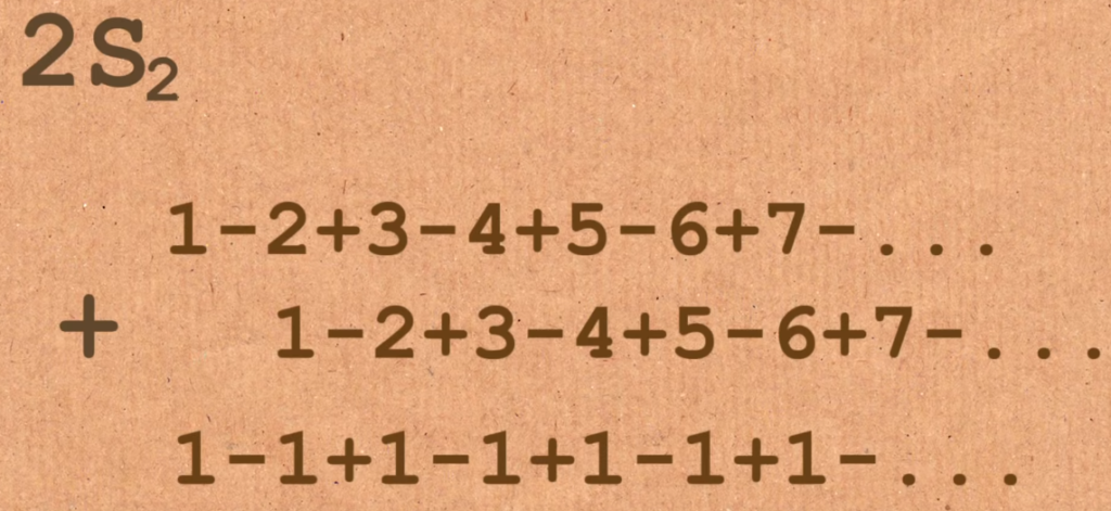
So indeed:
\[2S_2 = S_1\]
ergo
\[S_2 = \frac{1}{4}\]
And finally, the pièce de résistance. If we call the series of containing all natural numbers $S$:
\[S = 1 + 2 + 3+ 4+ 5+…\]
We can carry out the following calculation:
\begin{align*}S – S_2 &= (1+2+3+4…)-(1-2+3-4…)\\ &= 4 + 6 + 8 + … \\ &= 4(1+2+3+4…) \\ &= 4S\end{align*}
So now, a relatively advanced third-grader can tell you:
\begin{align*}S-S_2 = 4S\\ 3S = -S_2 \\ S = -\frac{1}{12}\end{align*}
This to me was shocking to say the least, and very shocking to say the most. What is perhaps even more unexpected is that this sum can be physically observed. We shall take a brief physical interlude, which in my opinion, will clear things up a bit. While I appreciate the sentiment that this video tries to convey, the mysteriously counterintuitive nature of maths, but for me, it served the exact opposite purpose.
Casimir Effect
Previously, we have established that QFT is in effect, an infinite collection of quantum harmonic oscillators. And indeed, this leads to the gratifying result that the energy of the vacuum, $\bra{0}H\ket{0}$ is simply an integral over all momentum modes and all of space. The Casimir effect is what happens when we disturb the vacuum.
Casimir, in 1948, performed the following experiment. He placed two parallel conducting plates (formally zero thickness and infinite area) into the vacuum. By changing the distance $d$ between the two plates, we vary the energy density, $\varepsilon$ of the vacuum, which would lead to a force between the plates, aptly named the Casimir force. The energy density of vacuum takes the following form:
\[\varepsilon = 2 \int \frac{\dd[3]{k}}{(2\pi)^3}\frac{1}{2}\hbar \omega_k\]
If we call the direction perpendicular to the plates $x$ and in order to maintain the continuity of our electromagnetic field at the conducting plates, the wave vector $\vec k$ can only take quantised values of $(\pi n/d , k_y, k_z) $, so we arrive at the expression for the energy density in between the plates:
\[\sum_n \int \dd k_y \dd k_z \frac{\sqrt{(\pi n/d)^2 + k_y^2 + k_z^2}}{(2\pi)^2}\]
This leads to a problem. What about the energy density outside the plates? This problem is overcome by introducing a third plate. We call the distance between the two outer plates $L$, and set it fixed. We can now move the middle plate and measure the force that way.
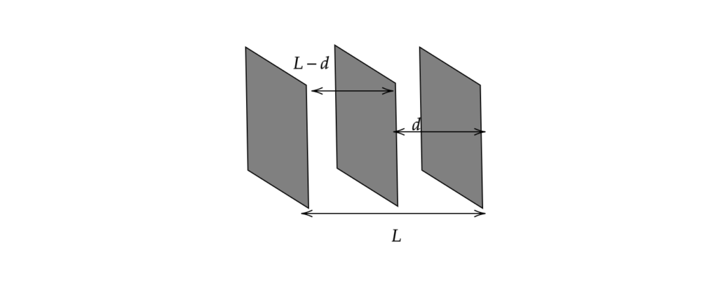
The energy $E$, can be found thusly:
\[f(d) = \frac{1}{2}\sum_{n=1}^\infty \omega_n = \sum_{n=1}^\infty \frac{n\pi}{2}\]
and that the total energy $E$ is:
\[E = f(d) + f(L-d)\]
The energy of the waves are simply given by the sum of all the frequencies (as the modes are given by standing sinusoidal waves). Also, we have conveniently set $\hbar=1$. Hopefully by now you would have realised, the energy tends to infinity, demonstrated by the infinite sum $\sum_1^\infty n$. To overcome this, we introduce a nifty trick, which I think is absolutely fantastic, namely:
Renormalisation Theory
What we can do is introduce an exponentially decaying factor $e^{-an/d}$, where $a$ parameterises some physics that we are not interested in at high frequencies. This in essence, picks out the ‘physically sensible’ parts of our system, the convergent part. We know what $a$ parameterise, it is the plasma frequency of the metal plates! Metal plates, depending on the material, can only keep waves up to a certain frequence before they start leaking out. The following then, will become our new $f$:
\[f(d) = \frac{\pi}{2d}\sum_{n=1}^\infty n e^{-an/d}\]
Now, we have a factor that tends to infinity, but we also have a factor that decays exponentially! To make sense of this, we can rewrite the above expression in another form:
\[f(d) = -\frac{\pi}{2}\pdv{a}\sum_{n=1}^\infty e^{-an/d}\]
which is in effect, the exact samething but expressed with a partial differential with respect to $a$. Reorganising the terms, we end up with:
\[\frac{\pi}{2d}\frac{e^{n/d}}{e^{n/d}-1}\]
To justify all of our hocus-pocus with introducing another factor $a$, we can simply say, let us set $a$ to 0!
Now, we can Taylor expand our $f$:
\[f(d) = \frac{\pi d}{2a^2} – \frac{\pi}{24d} + \frac{\pi a^2}{480d^3} + \mathcal{O}(\frac{a^4}{d^5})\]
Let us examine each term carefully. The first term, since we set $a\rightarrow 0 $, will tend to infinity, but the second term, being completely independent of $a$, will remain! In fact, discarding the parts that shoot off to infinity, we are only left with $-\frac{\pi}{24d}$!. And a short derivation from here:
\[F = -\pdv{E}{d} = -\frac{\pi\hbar c}{24d^2}\]
yields the force between the plates in SI units.
This is an astonishing result in my opinion. When faced with a divergent sum, at the beginning of this problem, we reassure ourselves that physics in nature don’t tend to infinity. Thus, we introduced a fudge factor $a$, which we encoded some physics (i.e. the plasma frequency of the metal plates) to essentially ‘pick and choose’ the convergent, sensible physics. Granted we had no reason to believe that such a force we are attempting to explain is indeed independent of the factor $a$ a priori, but the derivation would have taken a very different turn indeed should that have been the case.
Besides the ingenious renormalisation of our theory, the result directly showed that the sum of all natural numbers is indeed something we can observe in nature, and indeed we can… in the Casimir force!
In Zee’s book, he describes the fact that certain textbooks/people just brushing over the derivation by simply stating the sum of $n$ where $n\in \mathbb{R}^+$ is ‘appalling. So exactly what went wrong then?
Maybe it’s not so wrong…
With my very limited understaing of functional analysis, I shall attempt to explain how one can formalise this devilish sum in a mathematically rigid way.
The unintuitive nature of this subject is derived from the fact that we are working with what is effectively, infinitely dimensional vector spaces. Suppose we have a vector space $\mathcal{L}$, where
\[\mathcal{L} = \{(a_n)_{n=1}^\infty | a_n \in \mathbb{C}\}\]
$\mathcal{L}$ is the set of all possible infinity series of complex terms. It should be evident that $\mathcal{L}$ is a vector space, the telltale signs of a vector space do indeed apply to $\mathcal{L}$:
\[(a_n)_1^\infty \oplus (b_n)_1^\infty = (a_n + b_n)_{n=1}^\infty\]
this is just to say that when we add two infinite series together, we once again, get an infinite series.
Furthermore:
\[\forall \lambda \in \mathbb{C} , \lambda(a_n)_{n=1}^\infty = (\lambda a_n)_{n=1}^\infty\]
Suppose now we have a subspace, $\mathcal{C}$, a subspace of $\mathcal{L}$ containing those infinite series that are convergent, or in notation:
\[\mathcal{C} = \left\{(a_n)_{n=1}^\infty \in \mathcal{L} | \text{s.t. } \exists \lim_{n\rightarrow \infty} \sum_{k=1}^n a_k\right\}\]
I think it can be reasonablly inferred that $\mathcal{C}$ is also a vector space, i.e. as you add two convergent series together, the resultant series would also be convergent. We can say $\mathcal{C} \subset \mathcal{L}$
We have involved another entity in our definition of $\mathcal{C}$, and that is the $\lim$. If we think about it, the limit is nothing but a linear map, an operator that does the following:
\[\lim_{n\rightarrow \infty} : \mathcal{C} \rightarrow \mathbb{C}\]
In fact, the fact that $\mathcal{C}$ and $\mathcal{L}$ are related by a linear map would make $\mathcal{C}$ a dense subspace of $\mathcal{L}$.
And ultimately, what we are interested in, is to extend our linear functional (the limit as n goes to infinity) from $\mathcal{C}$ to $\mathcal{L}$, and Hahn-Banach Theorem will help us do exactly that.
Since both vector spaces are infinitely dimensional, we can approximate a point (a series in this case) in $\mathcal{L}$ by taking the sum of a sequence of points in $\mathcal{C}$, which would allow us to get infinitely close to any point in $\mathcal{L}$ from $\mathcal{C}$, in a topological sense.
In this topology of sorts, we can perhaps formalise, in a much more mathematically rigid way, some of the series used in Numberphile’s proof of the sum.
I shall return next week with Noether’s Theorem, and field theory in curved spacetime!
Leave a Reply